Genetic Population Structure of the Cownose Ray (Rhinoptera bonasus)
Cameron Neill
Governor’s School for Science & Technology
2011-2012
Mentor
Dr. Jan R. McDowell
Virginia Institute of Marine Science
1208 Greate Road, Gloucester Point, Va. 23062
Chesapeake Bay Hall, room N228
Abstract
The cownose ray, Rhinoptera bonasus, is a migratory ray that returns from the open ocean to two known nurseries, the Chesapeake Bay and the Gulf of Mexico, to reproduce. There are differing hypothesis about the genetic structure and status of the cownose ray population, due to lack of information. Using Sanger sequencing, information about the genetic structure of the two known nurseries was gathered. Analysis of this data suggests that there is isolated breeding between the Gulf of Mexico and the Chesapeake Bay, which at the minimum suggests that female rays return to the same nursery each year. Throughout the ND2 locus, there is an average genetic diversity of about 4%. Some genetic variation was found to be unique to one nursery; this enforcing the need for well-informed regulatory practices to protect the ray’s biodiversity as a fishery in one nursery could destroy irreplaceable biodiversity. From the data, the null hypothesis that there is no genetic divergence between the two nurseries and that the population is completely interbreeding was proven to be false with the alternate hypothesis that there is segregated breeding between the nurseries.
Introduction
 The cownose ray, Rhinoptera bonasus, is a migratory species of ray native to the Atlantic coasts of North and South America. Annually, the species travels to coastal nurseries to reproduce. The two known North American nurseries are the Chesapeake Bay and the Gulf of Mexico.
Recently, claims have arisen from the oyster industry that the ray population has increased to levels that are harmful for the prey species of the cownose ray; the ray mainly preys on shellfish, including oysters (Fisher 2011). The industry’s explanation for their claims is that the shark, the ray’s natural predator, has been fished to low levels and the cownose ray population is expanding without control or competition. Certain
factions wish to create a commercial fishery to control the population of the cownose ray, however not enough demographic and genetic information is known about the ray to accurately set quotas to protect the ray.
First and foremost, the International Union for Conservation of Nature, or IUCN, lists R. bonasus as near-threatened; this is in obvious conflict with the claims of a large population (IUCN 2011). In addition, the ray has only one pup per year (Neer
2005). This is only after the five to seven years that it takes to reach maturity. This low birthrate and schooling nature makes them extremely vulnerable to overfishing because the population may be caught in extremely high quantities that the low birthrate cannot sustain. The development of a fishery on the nursery grounds of the cownose ray may interrupt birthing and will kill newborn cownose rays as a by-catch. Finally, in the event of endangerment, the low birthrate will make it extremely difficult to recover to a safe population level. The situation at hand and the discrepancy over population status highlight the main issue regarding the cownose ray, which the IUCN states is the lack of information.
Information about the population status and structure must be gathered before any decisions are made, which is also high on the ICUN’s priorities. More information will also allow us to predict possible outcomes and monitor the ray populations for loss of genetic diversity. This information can be gathered by genetic analysis.
The first step in any genetic analysis is to gather DNA from samples. DNA isolation involves four main steps, lysis, binding, washing, and eluting (Rice 2010). Polymerase chain reaction, or PCR, is a method use to amplify selected portions of DNA. It is capable of taking a few copies of DNA and multiplying a selected strand to the thousands or even millions. The last major concept that was used is Sanger sequencing. Sanger sequencing is a method of visualizing the sequence of nucleotides in DNA strand.
 Using the methods of DNA extraction, PCR, and Sanger sequencing, information about the genetic population structure of the cownose rays was gathered. This involved analyzing the sequences of mitochondrial DNA collected and determining the relationships between female rays and young of year rays collected from the two breeding grounds. Mitochondrial DNA was specifically analyzed because it is solely passed maternally without recombination and is therefore generally easier to use to determine migration patterns than nuclear DNA. DNA sequences were used to infer the genetic structure between the two nurseries, the Chesapeake Bay and the Gulf of Mexico, and whether or not the populations are interbreeding or isolated. This was completed to determine if overfishing and population depletion in one nursery will harm just that population or the entire population. The haplotype relationship and divergence between the two populations was compared to test the null hypothesis that there is no significant divergence with the alternate hypothesis that there is significant genetic divergence. The null hypothesis suggests a completely interbreeding population, while the alternate suggests some form of geographically isolated breeding.
Methods and Materials
Tissue samples were collected by state and university sponsored fishing vessels from cownose rays caught in the Gulf of Mexico and in the Chesapeake Bay. The samples in this study were only taken from pregnant females, recent mothers, or the pups ensuring that the patterns inferred from the mitochondrial DNA would not be disrupted by any freely migrating males. From these samples, DNA was extracted using a DNeasy® Blood and Tissue kit (Qiagen, Valencia, CA) and the DNeasy spin-column protocol (table 1).
The isolated DNA was then used in a Polymerase Chain Reaction (PCR) to amplify select mtDNA loci. Individual primers were tested on a temperature gradient of
52-58 degrees Celsius to optimize the reaction, A standard PCR protocol was followed (table 2). Six total loci were tested: Cytochrome b, 12S subunit (CytB), Cytochrome c Oxidase 1 (COI), and NADH dehydrogenase subunits 2, 4 and 5 (ND2,4,5)(table 5).
After the PCR reactions are completed, a small aliquot of the product was visualized using gel electrophoresis to verify that there was product DNA present and that it was of the correct size. An aliquot of the master mix with no added template DNA was be mixed with dye and added into its own well to serve as a negative control. This was to ensure that DNA did not contaminate the master mix and that any results from correct amplification, not error.
Prior to sequencing, unincorporated primers and nucleotides were removed from the PCR product using a Qiagen QIAquick® PCR Purification kit (table 6). The purified product was then quantified using a Nanodrop spectrophotometer to determine the amount required for sequencing by measuring the amount and wavelength of light rays that pass through the sample.
After DNA quantification, a second PCR reaction, called a Sanger sequencing reaction was run (table 7). This reaction is similar to the first but with two exceptions. The first exception was that fluorescent ddNTPs are added along with the dNTPs; secondly, the forward and reverse primers were run separately for each sample. It must be noted that only the initial loci tests used both directions, in the final amplification of ND2 only the forward reaction was used due to poor quality reverse sequences in the initial tests.
After the sequencing reaction, another purification step was performed to remove any unincorporated reagents. However, instead of a Qiagen Kit, an ethanol precipitation was instead be used to purify and concentrate the PCR product (table 10). After completion the product was loaded into an ABI sequencer and a chromatogram, a
2d representation of the fluorescent markers measured by the sequencer, was produced
The chromatograms were viewed using Sequencher v4.10.1 (Gene Codes Corp, Ann Arbor, MI). The Sequencher program was then used to determine the validity of the chromatogram and to compare forward and reverse sequences from an individual to create a consensus. MacVector v8.0 (Accelrys Inc., San Diego, CA) was then used for aligning the DNA sequences generated from different individuals and creating both UPGMA and Neighbor-Joining trees. Both MEGA v4.0 (Tamura K, Dudley J, Nei M & Kumar S. 2007) and dnaSP v5.10.01 (Librado P. and Rozas J. 2009) were used to
analyze base genetic polymorphism. Parsimony trees were created using PAUP 4.0b10 (Swofford 2002).
The above methods were first completed for 5 loci with a subset of 8 rays from the Chesapeake Bay and 8 rays from the Gulf of Mexico to determine the most variable loci. After producing the UPGMA phylogenetic trees constructed based on the DNA sequence alignments by MacVector for the COI, CytB, ND2, ND4 and ND5 sequences the ND2 locus was chosen for expanded testing because it exhibited high variance and clear grouping between the Gulf of Mexico and the Chesapeake Bay. ND5 was immediately ruled out because of the extremely low variation of approximately 2 base pairs among all 16 sequences (figure 4). The COI locus had a low amplification success rate and CytB did not demonstrate clear relationships within the geographical locations (figures 1 and 2 respectively). The ND4 locus was variable and demonstrated clear grouping, however this locus was much more difficult to amplify than ND2 and
required several reamplifications to produce adequate PCR product (figures 3 and 5 respectively). ND2 was chosen because of the comparatively high level of sequence variation and clear geographic grouping while still remaining relatively easy to amplify. Thus the analysis of more samples was completed with the use of the ND2 locus.
Results
The research was a multistage project in the sense that the initial results were used to modify the methods in order to reach the final conclusion. The first stage of the research was the primer tests of COI, CytB, ND2, ND5, and ND4.
The COI primer test gave an 8 sequence alignment with two clades of sequences approximately 23 base pairs different (figure 1). The samples did show some minor grouping between the Chesapeake Bay and the Gulf of Mexico; however the sample size was too low to rule this out as being a random occurrence. The alignment from the Cytochrome B sequences was comprised of 14 different samples (figure 2). There was no clear grouping between geographic locations. The UPGMA phylogenetic tree created from the ND2 alignment contained 10 different samples and exhibited minor grouping at the lower clade of the tree (figure 3). The ND5 comparison tree was constructed from an alignment of 13 samples (figure 4). The tree suggested that the locus contained extremely low genetic variation. Finally, the ND4 locus was comprised of 10 samples divided into two haplotypes approximately 35 base pairs different (figure
5). The haplotypes almost exactly followed the geographic structure of the cownose ray samples.
The final research stage was the extended ND2 analysis. The final MacVector alignment was created from a total of 40 sequences which are 682 base pairs long. Overall there are four haplotypes, resulting in 3 distinct groups of sequences. The Gulf haplotype can be seen as blue on figure 6. The Bay haplotype is shown as yellow and the Mixed haplotype is green. Overall, the Gulf haplotype consisted of 12 sequences. The Bay and Mixed haplotypes numbered 3 and 25 sequences respectively. The Mixed haplotype was found in 9 rays found in the Gulf of Mexico and 16 rays found in the Chesapeake Bay.
Figure 7 has the three haplotypes divided into two evolutionary clades
approximately 58 base pairs different from each other. The UPGMA tree determined that the Bay and Gulf haplotypes were equidistant from the Mixed haplotype; however, the neighbor joining tree, a more flexible comparison, states that the Bay haplotype is 3 base pairs more distant from the Mixed Haplotype (figures 7 and 8 respectively). The neighbor joining result is more supported by statistical and base pair analysis (table 12).
Table 12 was created from analytical data produced from dnaSP v5.10.01 and MEGA v4.0. Average genetic divergence and diversity are measured in average base pair differences per total number of base pairs. It was found that between the Mixed and Gulf haplotypes the average nucleotide divergence is 0.093; between the Mixed and Bay haplotypes there is an average nucleotide divergence of 0.099. Between the Gulf and Bay haplotypes there is an average nucleotide divergence of 0.029. This equates to a 9.3%, 9.9%, and a 2.9% divergence respectively. The average nucleotide divergence between the Chesapeake Bay and the Gulf of Mexico geographic locations is 0.054. The probability that this was a random occurrence has a P value of less than 0.0001. Within geographic groups, the Gulf of Mexico and the Chesapeake Bay have an average nucleotide diversity of 0.048 and 0.028 respectively. Both programs were used to calculate the total nucleotide diversity. MEGA estimated the diversity at 0.047 while dnaSP calculated it to be 0.04268. These results, while different, suggest that on average
2 randomly selected cownose rays are 4% different.
Discussion and Conclusions
From the UPGMA tree created by MacVector and the parsimony tree created by PAUP of the 40 sequences, it is suggested that the Chesapeake Bay and the Gulf of Mexico are genetically distinct. Within the Gulf of Mexico there are two separate haplotypes while in the Chesapeake Bay there is predominately a single haplotype. This level of divergence and segregation between the haplotypes is indicative of a past isolation event that caused the ND2 locus to mutate separately between the two
locations. The major haplotype of the Chesapeake Bay is also present in the Gulf of Mexico; this suggests that following the isolation event there was a one way migration of rays from the Chesapeake to the Gulf of Mexico. Analysis showed that there is on average a 9.3% (table 12) difference between the Gulf and Mixed haplotypes. Utilizing a commonly accepted rate of animal mutation of 2% per 1 million years it can be estimated that the two ray populations were isolated for about 4.5 million years based on this locus (Brown, George, Jr, and Wilson.1979). However, it must be noted that sharks and rays are thought to have much lower mutation rates than other animals and it is likely that the true length of isolation is much higher.
In addition, there is a haplotype present in the Chesapeake Bay that is much more closely related to the Gulf haplotype than to the Mixed haplotype. Between the Gulf and Bay haplotypes there is an approximate 3% (table 12) difference which suggests that the two have been isolated for about 1.5 million years. Due to the divergence between the haplotypes, the results suggest that 1.5 million years ago rays from the Gulf of Mexico migrated to the Chesapeake Bay at which point they became isolated from each other. This time frame agrees with the last known ice age, which occurred about 1.5 million years ago; it is possible that a migration corridor was closed during this period. This is a much more speculative result, however, due to the low number of rays found to have the Bay haplotype. To test this theory, a larger sample size would have to be analyzed.
With regard to the hypothesis and original goal of the project, the null hypothesis has been proved to be false. If the population of cownose rays was completely flowing and interbreeding then all haplotypes, regardless of the base pair sequences of the haplotypes, would be evenly dispersed between the Chesapeake Bay and the Gulf of Mexico. This is simply not suggested from the data.
The sequences tested were from mitochondrial DNA which is only passed down
maternally, the father plays no role. The data suggests that at the bare minimum the female rays return to the same nursery to pup each year. This suggests a segregated breeding population. With this in mind and with the information that most females are pregnant before leaving the birthing grounds each year (Chesapeake Bay Program 2012) the data suggests that the population of cownose rays is fairly segregated to the two breeding grounds with minimal interbreeding. However, this result does not account for the migratory patterns of the males and it is possible that there is male-mediated gene- flow. The only way to test the male gene-flow and thus the overall genetic relationships would be to examine nuclear DNA.
In the context of the conservation of the rays, overall there is an approximate
4% diversity within the mitochondrial ND2 locus of the population, with a 5.4% divergence between samples from the Gulf of Mexico and the Chesapeake Bay. This level of divergence is significant with a p-value of <0.0001 (table 12). From this study, added onto the risks of extinction is the risk of destroying unique genetic diversity, through the loss of alleles and haplotypes, that cannot be recovered. Not only would the destruction of a nursery ground cause a severe loss in evolutionary potential, but also it is suggested by the data that due to the low cross migration rates the population might never be restored, certainly not within our lifetimes.
Acknowledgments
I would like to thank Dr. Jan McDowell for being my mentor. She has taught me the concepts of the project and has facilitated my research. In addition, Kristy Hill also taught me how to do most of the procedures required by my project. They both have helped to revise this paper along with performing some procedures such as PCR
and gel electrophoresis. The various collectors, including Dr. Fisher, provided the tissue samples for my analysis.
Literature Cited
Accelrys Inc., San Diego, CA. Version 8.0
Brown, George, Jr, and Wilson.1979. Rapid evolution of animal mitochondrial DNA.
Procedings of the National Academy of Science. vol. 76 no. 4 1967-1971. Chesapeake Bay Program. 2012. Cownose Ray.
http://www.chesapeakebay.net/fieldguide/critter/cownose_ray
Cold Spring Harbor Laboratory. n.d. Polymerase Chain Reaction. DNA Learning Center http://www.dnalc.org/resources/animations/pcr.html
Fisher, R., G. Call, and R. Grubbs. 2011. Cownose Ray (Rhinoptera bonasus) predation relative to bivalve ontogeny, Journal of Shellfish Research 30: 187-196.
Gene Codes Corp., Ann Arbor, MI. Version 4.10.1
IUCN. 2011. Rhinoptera Bonasus. IUCN Redlist. http://www.iucnredlist.org/apps/redlist/details/60128/0
National Diagnostics. 2010. Sanger Sequencing. http://www.nationaldiagnostics.com/article_info.php/articles_id/21
Neer, J. and B. Thompson. 2005. Life History of the cownose ray, Rhinoptera bonasus, in the northern Gulf of Mexico, with comments on geographic variability in life history traits. Environmental Biology of Fishes 73: 321-33.
Qiagen Inc., Valencia, CA. 2006 version.
Rice, G. 2010. Montana State University. Microbial Life Educational Resources. DNA Extraction. http://serc.carleton.edu/microbelife/research_methods/genomics/dnaext.html
Saitou, N., and M. Nei. 1987. The neighbor-joining method: a new method for reconstruction of phylogenetic trees. Molecular Biology and Evolution 4:406-
25.
Swafford, D. 2002. Florida State University.
Tamura K, Dudley J, Nei M & Kumar S. 2007. MEGA4: Molecular Evolutionary Genetics Analysis (MEGA) software version 4.0. Molecular Biology and Evolution 24: 1596-1599.
Thompson, J.D., D.G. Higgens, and T.J. Gibson. 1994. Custal W: improving the sensitivity of progressive sequence alignment through sequence weighting, position-specific gap penalties and weight matrix choice. Nucleic Acids Resource 22: 4673-80.
Table 1 – DNA Isolation Protocol
Add 180 µl of the Qiagen buffer ATL to each labeled 1.5 ml microcentrifuge tube.
Cut 25 mg from each sample of tissue and wash with DI water. Mince and add to the microcentrifuge tubes
Pipette 20 µl of proteinase K to each of the tubes. Vortex to mix.
Incubate samples at 56 °C for 1-3 hours to overnight. After the tissue is completely lysed, mix by vortexing.
Combine 200 µl of the buffer AL and 200 µl of 100% ethanol per sample. Mix thoroughly and add 400 µl of the solution to each sample tube. Vortex samples.
Pipette mixture into a DNeasy® spin column. Centrifuge at approximately 8000 rpm for
1 minute. Discard flow-through.
Add 500 µl of the Qiagen buffer AW1 to each sample. Centrifuge again for 1 minute at
8000 rpm. Discard flow-through.
Add 500 µl of the Qiagen buffer AW2 to each sample. Centrifuge for 3 minutes at
14000 rpm. Replace collection tube with 1.5 ml microcentrifuge tube.
Pipette 200µl of Qiagen buffer AE onto the DNeasy column filter. Incubate at room temperature
Centrifuge at 8000 rpm for one minute. The flow through is usable DNA.
Table 2 – PCR Protocol
Create master mix by combining the correct reagent volumes (table 3)
Add the required amount for four more reactions for the negative control and to account for pipetting error.
After creating the master mix, pipette 4.7 µl of the solution into each tube. Next, add 0.3 µl of template DNA to each tube.
For the negative control, add 5 µl of the master mix into a separate PCR tube. Load strip tubes into BioRad Cl000 thermocycler.
Run program as shown in table 4.
| Table 3 – PCR Reagents | |
| Reagent | Volume for one reaction (µl) |
| PCR H2O | 2.975 |
| BSA (1mg/ml) | 1 |
| PCR Buffer (10x) | 0.5 |
| dNTP (10 mM each) | 0.1 |
| Forward Primer (100 µM) | 0.05 |
| Reverse Primer (100 µM) | 0.05 |
| Taq polymerase (50 U/µl) | 0.025 |
| Total volume for one reaction: 4.7 µl |
Table 4 – PCR Thermocycler Program
| Step | PCR Process | Temp (°C) | Time (minutes) | Cycles |
| 1 | Initial Denaturation | 94 | 5 | 1 |
| 2 | Denaturation | 94 | 1 | 35 |
| 3 | Annealing | 56* | 1 | 35 |
| 4 | Extension | 72 | 1 | 35 |
| 5 | Final extension | 72 | 7 | 1 |
| 6 | Final hold | 4 | Forever | ∞ |
| *ND2 – 65 | *ND4 – 58.7 | *ND5 – 58.7 |
Locus
(Mitochondrial)
Primer Primer Sequence
Cytochrome B Rb_Cytb_F 5’GGCCTHTTYCTRGCTATACACTACAC3′
Rb_Cytb_R 5’AGGGRTGGAATGGRATTTT3′
12S 12SF22 5’GCATGGCACTGAAGATGCTAAGATGA3′
16SR2600 5’AATCGTTGAACAAACGAACCCTTAATAGC3′ COI CsquCO1F 5’TCGACTAATCATAAAGATATCGGCAC3′
CsquCO1R 5’TAGACTTCTGGGTGGCCAAAGAATCA3′ ND4 Rhin_ND4_F1 CTTCCCATTCCTAATCYTRGC
Rhin_ND4_R2 TATGTTCTCGKGTGTGGGA
ND5 Rhin_ND5_F1 CATGTYAAAACAGCYGTAAAAACC Rhin_ND5_R3 TTTTCGGATATCTTGTTCATCATTTA
ND2 Rhin_ND2_F1 GAACCCYTTAATCCTCTYCATC Rhin_ND2_R3 ATRGGGGTTAATGGRAGRAG
Add 25 µl of Qiagen buffer TB to each PCR product.
Load samples into QIAquick columns and place in a vacuum manifold. Apply vacuum. Add 750 µl of Qiagen buffer PE to each column. Apply vacuum again.
Transfer each QIAquick column into a 1.5 ml microcentrifuge tube. Centrifuge at
13,000 rpm for one minute to remove residual ethanol.
Place each column into a new microcentrifuge tube and add 50 µl of Qiagen buffer AE. Centrifuge for 1 minute at 13,000 rpm. Flow-through is purified product.
Combine all reagents into a single master mix according to volumes listed on table 8.
The 1/8 ABI protocol was utilized for the samples.
Add 4 µl of master mix to each tube (the forward and reverse primers are completed as separate samples).
Add 1 µl of the purified PCR product to each tube.
Place tubes into a thermocycler and use the program listed in table 9.
| Dilution | BigDye | 5X Buffer | Primer | Template | Water |
| 1/8 ABI | 0.25µl | 0.875µl | 0.32µl | 1µl | To 5µl |
| 1/32 ABI | 0.0625µl | 0.96875µl | 0.32µl | 1µl | To 5µl |
| Step | PCR Step | Temp (oC) | Time (seconds) | Cycles |
| 1 | Initial Denaturation | 96 | 60 | 1 |
| 2 | Denaturation | 96 | 10 | 25 |
| 3 | Annealing | 50 | 5 | 25 |
| 4 | Extension | 60 | 240 | 25 |
| 5 | Final Hold | 4 | Forever | ∞ |
Table 10 – Ethanol Precipitation Protocol
Combine correct amount of reagents according to table 11, in this study the 5 µl protocol was utilized. A few extra reactions should be added to the master mix to
account for pipetting error.
Add appropriate amount of master mix to each tube. Invert tubes to mix. Incubate at room temperature for at least 15 minutes.
Centrifuge for 30 minutes at 2000-3000 g.
Cut off lids and invert over paper towels in centrifuge. Centrifuge at 50 g for 1 minute. Add 37.5 µl of 70% ethanol to each tube. Invert tubes to mix. Centrifuged again at
2000-3000 g for 10 minutes.
Remove lids and invert tubes again. Centrifuge at 50 g for one minute.
Cover with Kimwipes and leave to dry in the dark at room temperature for 10 minutes. Add 20 µl of Hi-Di Formamide to each tube
Use a thermocycler to denature the DNA for 2 minutes at 95 degrees Celsius. Pipette ten microliters of each sample will be placed into a 96-well plate.
Table 11 – Ethanol Precipitation Reagents
Reagent Volume to precipitateVolume to precipitateVolume to precipitate
20µl of sequencing10µl of sequencing5µl of sequencing
reaction
reaction
reaction
3M sodium acetate 3µl 1.5µl 0.75µl
Non denatured 95%62.5µl 31.25µl 15.625µl
ethanol
Deionized water 14.5µl 7.25µl 3.625µl
Total: 80µl 40µl 20µl
Table 12 – Statistical and DNA analysis
Average genetic divergence between haplotypes.
| Haplotype
Mixed |
Mixed
0 |
Gulf |
Bay |
| Gulf | 0.093 | 0 | |
| Bay | 0.099 | 0.029 |
0 |
| Average genetic divergence between geographic locations. | |||
| Locations
Chesapeake Bay |
Chesapeake Bay
0 |
Gulf of Mexico | |
| Gulf of Mexico | 0.54 | 0 | |
Probability of randomly choosing two different haplotypes: 0.586 or a 58.6% chance
Total nucleotide diversity: dnaSP 0.04268 MEGA 0.047
P value corresponding to the above data p <0.0001
Estimates of average evolutionary divergence within geographic groups.
Gulf of Mexico 0.048
Chesapeake Bay 0.028
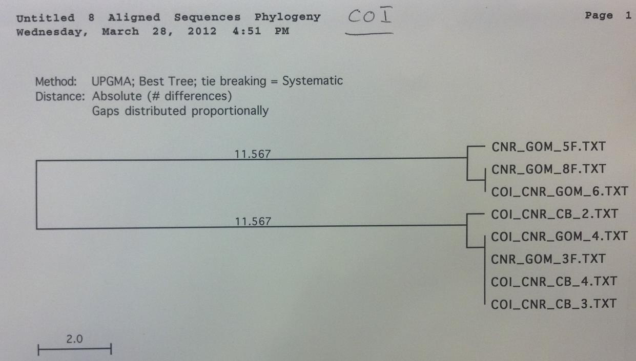
Figure 1. COI sequence comparison tree. Note that sequences are grouped between the Gulf of
Mexico and the Chesapeake Bay, however there is a very low amplification success.
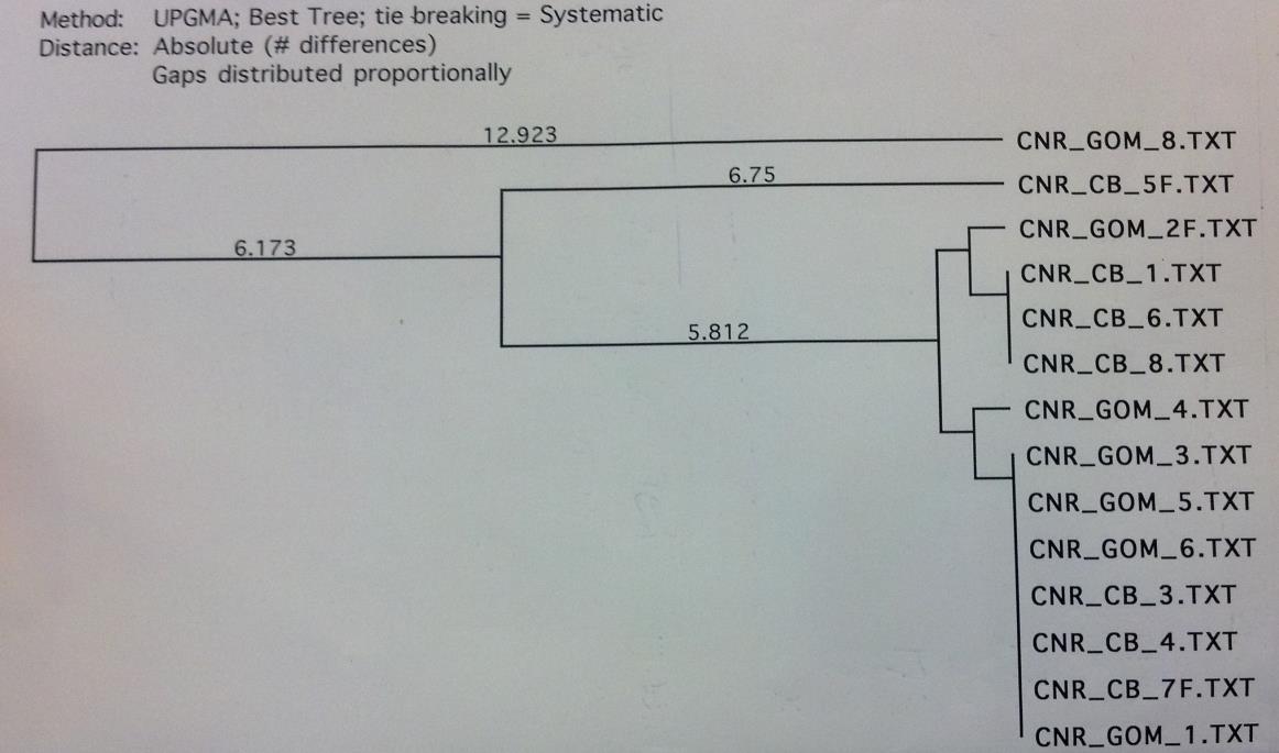
Figure 2. CytB sequence comparison tree. There is no significant haplotype grouping between geographic locations.
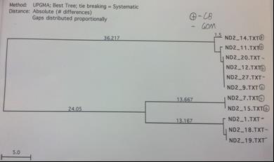
Figure 3. ND2 sequence comparison tree. Pluses denote the Chesapeake while minuses denote the Gulf. Note the grouping within geographic groups on the bottom clade.
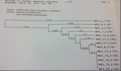
Figure 4. ND5 sequence comparison tree. Note the extremely low variance, as denoted by the numbers on the horizontal lines. Pluses denote samples collected from the Chesapeake Bay while minuses denote rays collected from the Gulf of Mexico.
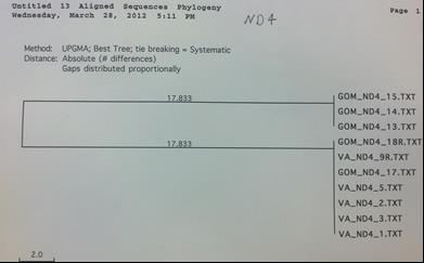
Figure 5. ND4 sequence comparison tree. There is clear grouping between two distinct haplotypes. The upper clade consists of only Gulf rays while the lower clade has a Chesapeake Bay majority.
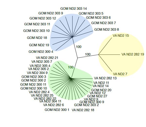
Figure 6. Bootstrap tree created using 1000 repeats and 100 random replicates. It was created using parsimony, the idea of using the lowest number of base pair mutations from a common ancestor to estimate relationships. The Gulf haplotype is blue, the Bay haplotype is yellow, and the Mixed haplotype is green.
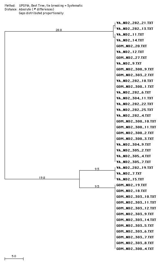
Figure 7. UPGMA phylogenetic tree created using MacVector.
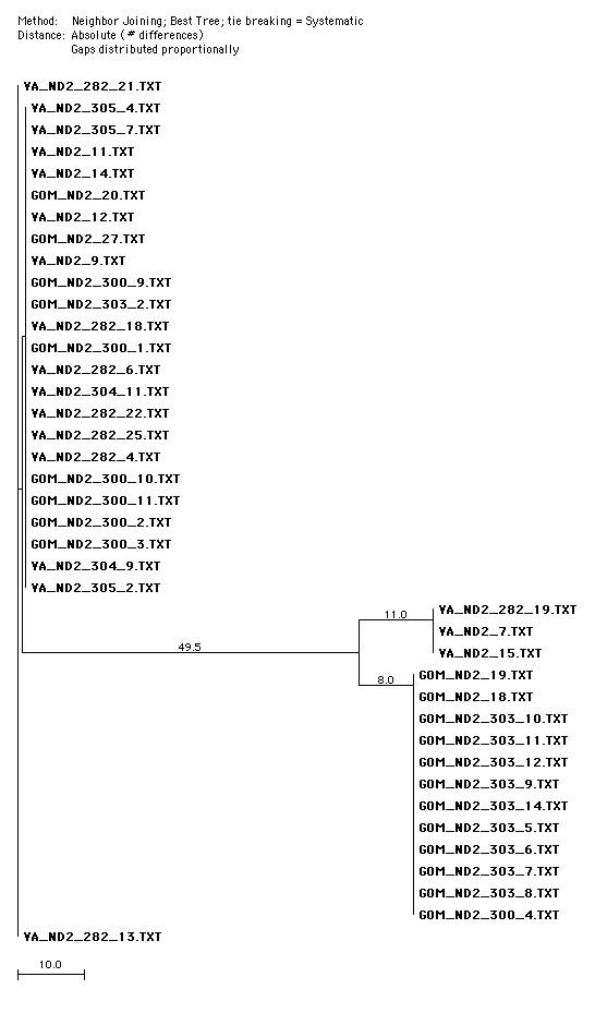
Figure 8. Neighbor-Joining tree created with MacVector. Note that the Bay haplotype is more distant from the Mixed haplotype than the Gulf haplotype. This suggests that the Bay haplotype were originally from the Gulf haplotype and have since genetically diverged.
Cameron Neill
York High School – York County School Division
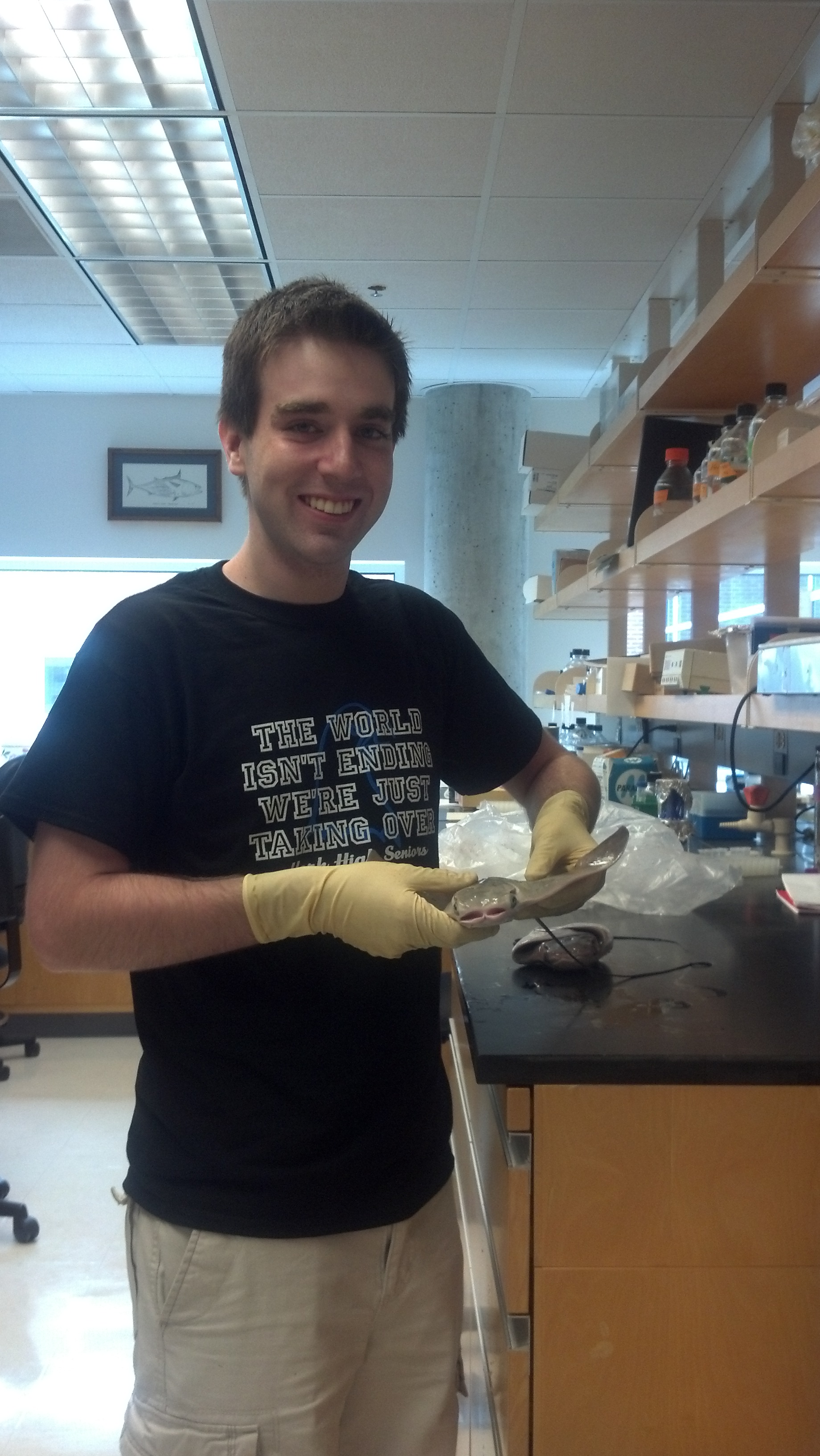
“For my mentorship, I worked in the Fisheries Genetics lab at the Virginia Institute of Marine Science. During my mentorship I learned many concepts surrounding DNA analysis and spent extensive amounts of time analyzing the DNA of cownose rays to study migration and reproductive patterns. It was a great experience for me; I wouldn’t have changed a thing. I hope the same for my mentor Dr. Jan McDowell and lab technician Kristy Hill, both of whom taught me everything I know about the field. My biggest take – away is that things will always go wrong in science; all you can do is try again.”
|
|
 Cameron will pursue a degree in aerospace engineering at Georgia Institute of Technology beginning this fall. He has greatly appreciated his opportunity to participate in the Governor’s School and his mentorship and recommends the program to all who have the opportunity.
You are truly a man after my own heart! I loved your report especially the way you folowed the Scientific Method! Keep up the great work, Cameron, we are very proud of you!